Wednesday, May 16, 2007

6th Assignment- Volume Conversion Table & PowerPoint


Investigate:

According to the book Civilization One, ancient civilizations worked out a system of measurement based on pendulums and the passage of time, measured by astronomy. From historical information it shows that the ancient civilizations likely created consistent measuring units. These units were based on a pendulum that would make a specified number of sweeps during the time it took to track the course of the planet Venus. Between two pillars set up exactly one degree of a circle apart was where the pendulum was located. All our modern measurements like the Metric System and the English Units are based on the findings of the ancients. These modern units are thought to be from this same system.

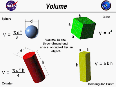
One of the most useful types of measurement is volume. The dictionary describes Volume as the amount of space occupied by a three-dimensional object in cubic units or in units that measure liquids. Arithmetic formulas are used to calculate the volume of straight-edged and circular shaped objects. To find the volume of an object you have to divide its mass by its thickness (density). Volume is used a lot in thermodynamics (the study of the relationships between heat, work, and energy), pressure, cooking, area, density, in the trade market; like with oil, and in construction. It is a big part of the world that we live in today.

My assignment was to design a conversion table that converts measurements of volume in mathematics using Excel and to then make a PowerPoint presentation that describes what I did. This is a useful skill to learn because there are many measurements all over the world and it is necessary to know how to convert them. I went to many different websites that made conversions for me and they told me how much one unit of measurement was. This was the first piece of information I needed to start my project. Once I knew this, I thought of all the information I had taken in over the year and I made up a formula to that converts on unit to another. What I did was I put =PRODUCT(A2*n). The number in cell A2 would always be the starting measurement; litres. N meant the amount the starting unit must be multiplied by to get the amount of the other unit. If I added a number to the starting unit it could convert it to any other measurement. I used to most common measurements of volume in my table because there were too many measures in all for me to do, most of which not many people know of. I used litres, tablespoons, ounces, pints, quarts, gallons, millilitres, kilolitres. A method I used to check if my table was correct was to go on to the yahoo for kids conversion table which was able to convert the measurements for me. So when I would put in one litre and convert it to pints, for example, in the yahoo conversion calculator and in my conversion table the result was the same. I checked this same way with all of my units.


Design:

When I was thinking of how my conversion table would look I was kind of confused whether it should be horizontal but I decided to do it lengthwise because it would be simpler. I thought this because I would only have to be able to convert one measurement to another at one certain period of time instead of all of them at the same time, as I would have to if I did it horizontally. I also decided to give it a bit of colour by making it pink so that it would look a little more interesting.


Plan:

Here are the steps that I planned to take before I made my conversion table:

  1. Find the history of the measurement system especially when it comes to Volume. I got this information from the websites (http://www.crosswalk.com/homeschool/1464307/page2/), and (http://www.answers.com/Volume).
  1. Relate Volume to everyday life and explain why it is important that we know how to convert measurements. I thought about where in life I as a person have seen or hear that volume has been used. I also got information from the same two websites that I mentioned before. These two steps should be done in about two days, possibly adding bits of information I may find as I go along.
  1. Find a formula that was the base of the conversion table. I researched in as many websites as I can and I can also use excel help.
  1. As I said before I can find out how much each measurement was worth on the yahoo kids converter on the website (http://kids.yahoo.com/reference/index). I knew about this website from beforehand.
  1. I then to make conversions from litres to different units, I find how many of the other units equalled a litre. For example, 100 kilolitres equals one litre.
  1. Next I punch in the numbers into my formula. =PRODUCT(A2*n). The product, when I was trying to convert litres to kilolitres, should look like this: =PRODUCT(A2*1000).
  1. Afterwards repeat step 7 so that you can convert all the units from litres to pints, quarts, kilolitres, etc.
  1. Create a PowerPoint presentation basically explaining what volume is, why it’s important in everyday life and how I made my conversion table.

Comments on the Plan:

I just could not find how to make a conversion table for Volume so I resorted to my own knowledge of how Excel works. So I made the formula using my own common sense. I hope that this plan will be successful in the completion of the conversion table.


Create:

I made my conversion table following the steps that were outlines in my plan earlier. I finished making the conversion table using Excel and the PowerPoint slide show was obviously made in PowerPoint.


Evaluate:

I felt that the conversion table was a success but I was confused because I didn’t know if I had to convert the most used measurement to all the other measurements or if I had to make the conversion table work so that it converted any measurement to another, but I stuck with my original idea. I just made the conversion table convert the most used unit of measure meant to the others. I tested the conversion table and it worked how I planned in all occasions. Anytime I put a number into the first unit it would automatically convert it into the amount of the other units it would equal.

However, some improvements that might have been done would have been to make my original idea for the conversion table and to try the other way, which was to make the conversion table work so that it converted any measurement to another. I could have done two tables and compared them. The biggest difficulty I found when doing this project was that it was extremely hard to find information that could help me make the conversion table and the little information that I did find was very difficult to understand it was all written in English that was difficult; using technological terms that I did not understand. If I had not had past knowledge about Excel I would not have been able to do anything with this project. I felt very worried during the design cycle and I was not completely happy with how it turned out but I did as well as I could. I felt happy with the PowerPoint though. I found many good pictures and I was very familiar with PowerPoint so I knew many things to enhance my slideshow to make it more interesting.

From this project I learned that Volume is a very important thing in everyday life, that there are many measurements for Volume, and that Volume has developed al lot over the years from how the ancient civilizations found Volume to how modern mathematician find volume. It is necessary to know how to convert the volume measurements especially when it comes to the import and export, for example with oil. The volume of the oils is in different measurements depending on the country. So, it would be important to know how to convert it.
Monday, March 12, 2007

5th Assignment- Interactive Grade Book Using Excel

Investigate: I found most of my information from Excel help and the website (http://www.internet4classrooms.com/excel_grade.htm) and this source was very useful but it didnt give me all the information I needed. I got part of the imformation for Excel help. With Excel help that was the part that helped me make the gradebook interactive. This assignment is very useful to teachers around the world because it makes it easier to organize the grades of each of the students, find averages, and find the total grade for the quarter or maybe year that the student deserves. When investigating I was asked to look for information on how to make the gradebook and I wanted to know how, especially, to make it interavtive so that the final grade depends on tthe other averages. My guiding question was...How do you make an interactivce grade book using Excel?


Design:
To make the basic design of my grade book I just followed the directions of the website but to give it a personal touch I made each column in different shades of purple.

Plan:

ENTER DATA

To make a spreadsheet of students' grades:

  1. I opened a new spreadsheet: Click Microsoft Excel on my desktop or in the Start menu. (You also might find Excel in Start>Programs>Microsoft Office>Microsoft Excel.)
  2. The new spreadsheet is made up of many small squares; those squares are called cells. The cells are arranged in columns across the top of the spreadsheet (A, B, C…) and in rows down the left side of the spreadsheet (1, 2, 3…). The top left cell in the spreadsheet is cell A1.
  3. I clicked in cell A1 and typed Names. Then I hit Enter
  4. I then clicked in cell A2, typed a student's name, and then I hit Enter.
  5. In cell A3, I typed another student's name, and hit Enter. I continue down the page until all 14 students' names were entered.
  6. I clicked in cell B1 and type a name for the assignment I was recording, (vocabulary test). Hit Enter.
  7. In cell B2, I typed the first student's grade and I hit Enter.
  8. In cell B3, I typed the second student's grade and I hit Enter.
  9. Continue down the page until all students' grades are recorded.
  10. I clicked in C1 and typed the name for the other assignment whose scores I was recording, (Marketing Test). I then hit Enter.
  11. In cell C2, I typed the first student's grade on the Marketing Test and then hit Enter.
  12. In cell C3, typed the second student's grade on the Marketing Test and then I hit Enter.
  13. Continue down the page until all grades are recorded.
  14. Next I found the average for these two grades for each student.

USE A FORMULA
To average each student's grades:

  1. Click File in the Excel menu bar and choose Save. Open the folder in which you want to save your file. Type a name for the file in the File Name blank. Click Save.
  2. Click in cell D1 and type Current Average. (Don't worry if the words "bleed" into cell E1; just double click the line between the letter D and the letter E at the top of the spreadsheet and the column will automatically resize!)
  3. Click in cell D2 and type =(B2+C2)/2. Hit Enter. The first student's average grade. Why? The formula =(B2+C2)/2 told Excel to add the numbers in cells B2 and C2 and then divide the sum by 2.)
  4. Click in cell D2. Hold down the mouse button to highlight the rest of the students' grades. Release the mouse button.
  5. Click Edit and choose Fill and Fill Down. (You don't have to retype the formula.) An average of each student's grades now should appear.

I did this for each of the students and I found averages for each of the different types of assessments: Tests, Participation and Projects. So I got three different averages. I then multiplied the average by how much percent of the total grade each kind of assessment was worth. Tests were worth 40%, Participation was worth 10%, and projects were worth 50%. For example on the Marketing test I multiplied the average 93 by 0.4 to get the percent because tests were worth 40%. I did the same method for each of the three kinds of assessments. For Participation I got the grades for homework and quarter participation found the average and multiplied that average by 0.1 because participation was worth 10%. I then found the grades for projects, found the average and then I multiplied this average by 0.5 because projects were worth 50%. I put all of the averages in different columns that correspond with which type of assessment they are related to. I also did that with the percentages.

Once I had found all the percentages I made a new column at the end (Column L) and I added all the percentages together to get the class grade. I called this column class grade. The formula I used was (=E2+I2+K2). This means that u added the percent in column E, the percentage in column I, and the percentage in column K. Then I figured out how to find out what the letter grade for the percentage was. To do so I went to Excel Help. It gave me an example of the formula to use. I copied it but I substituted the grades with my percentage grades and I put in the letter grades this percentage grade would be worth. This was the formula I used: =LOOKUP(L2,{94.5,98.45,80.15,85.35,87.5,86.55,94,88,98.6,87.45,80.75,64.6,88.7,94.95},{"A",
"A+","B-","B","B+","B+","A","B+","A+","B+","B-","D","B+","A"}). I did this for all the students but this was in column N that was named final grade because in column M it was the basic grade with minus and plus letter grades but in column N it had the plus and the minus'. For example, in column M the grade would be an A but in column N the grade would become and A+.

Conclusion:

I found this assignment very difficult. It was hard for me to find the information I needed because I didn’t understand the instructions very well because of the language used. A lot of the times I just copied the formulas but I didn’t really understand them. It took me a long time to really understand how to do it and I had to ask for some help. This was something that I had never done before so many techniques were new to me. The solutions to most of my problems with this project came from me looking in Excel help and trying many different things to find and answer. I don’t think that I will be using these techniques very much in the future but it is useful to know.

This assignment was assessed with MYP criteria.


Friday, February 16, 2007

4th Assignment- Interactive Crossword Puzzle

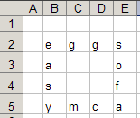
In this class I was given the task of making a interactive crossword puzzle using Excel that is kind of like a game to teach the ESOL students new vocabulary. I sued the instructions below from the website (http://www.internet4classrooms.com/excel_puzzle.htm) to make it.

Open Excel and type the letters above in the same places you see them. [I made the columns narrow, but you can wait on that]

  • Click on the letter A in gray (column heading), leave your mouse button depressed and drag over to column heading F.
  • Put your cursor on the line between any two column headings, click and drag until Excel informs you that you have a column width of 7.00 (54 pixels).
  • Click on the number 1 in gray (row heading), leave your mouse button depressed and drag down to row 6.
  • Put your cursor on the line between any two row headings, click and drag until Excel informs you that you have a column height of 37.50 (50 pixels).
  • Click on the letter E in cell B2, leave your mouse button depressed and drag to the letter a in cell E5. All letters should now be highlighted.

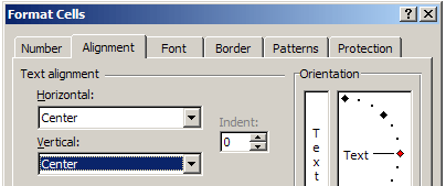
  • From the Format menu select Cells, then select the Alignment tab
  • Select Center alignment from both the Horizontal and Vertical blocks.
  • Click on the Font tab, and select 24 in the size box.
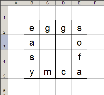
  • Click on the Border tab. Select Outside and then also select Inside. Click OK.

The next step will be to color all of the squares without letters in them.

  • Click in cell A1 (on your Excel worksheet, not on the picture above), depress the Ctrl key and leave it depressed until you have clicked on all squares that do not have letters in them. If you click and drag you must release the mouse button at the end of a line (but do not release the Ctrl key). Now click and drag another line of cells, until all are highlighted. (Note: The last cell selected will be outlined in black, but not filled with the highlight color. It is selected)
  • Release the Ctrl key (but do not click on the worksheet), and click on the Fill Color button on the Formatting toolbar. [I selected yellow.]

Two steps to go! Next you will add comments at the starting letter of each word, to serve as a clue to the word.

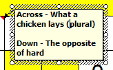
  • First, the letter e. This one will require a clue for across and a clue for down. Put them in the same comment with an empty line between the two clues.
  • Right-click the letter e (in cell B2) and select Insert Comment. Highlight anything that is already in the comment box and type the clues.
  • Continue until you have clues written for each word.

Final Step! This step is what makes the puzzle interactive. If a student types the wrong letter in a box, the letter will turn red when the student hits the Enter key. This process is called setting conditional formatting.

  • Click on the letter e in cell B2.
  • From the Format menu select Conditional Formatting.
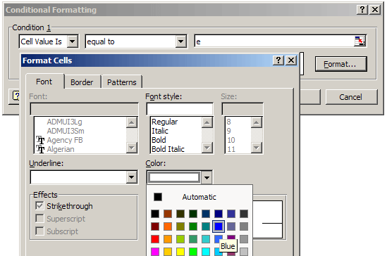
  • In the Condition 1 window change the middle box to "equal to" and in the long box to the right type the letter e.
  • Select the Format button and select a color you wish to use for correct letters. Some people use green (for Go) but I think blue shows up better.
  • Click OK.

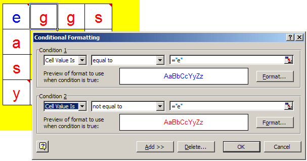
  • With the Conditional Formatting window still open, click the button labeled Add >>.
  • In the Condition 2 section, select "not equal to", type the letter e in the box to the right and select the Format button to select the color Red for incorrect letters.
  • Click OK. The letter e turns blue.
  • With the letter e still selected find the Format Painter button on the Standard toolbar. It looks like a paint brush.
  • Double-click the paint brush.
  • One at a time, click on each of the other eleven letters. ["Trust me, there is method to my madness."]
  • Each of the other letters should now be red, because they have been formatted incorrectly. Right? [Psst! The answer is "Right!"]
  • Select the letter g in cell C2
  • From the Format menu, select Conditional Formatting. See what pops up? See the Method in my Madness?


The crossword was assessed by the criteria in Design Technology and Computer Tchnology in the MYP Program.

A. Investigate: As I said before, we were assigned to make and interactive crossword puzzle and I got my information on how to make it from http://www.internet4classrooms.com/excel_puzzle.htm.

B. Design: In my crossowrd puzzle, I made it so that when you type in the wrong letter it will trun red and when you type in the correct letter it would turn blue. The background around the letters that are in the cells was black. I chose this baclground colour so that the colours would stand out more.

C. Plan: In planning my crossowrd I found random 10 words from the dictionary that I thought were at the level of the ESOL students and I got the definition of them, them wrote them down. These words were prosperity, conceal, divulge, pacifist, sooth, miser, miscellaneous, demeaning, vivify and affection. By doing this I knew exactly what words I wanted to put in my crossword puzzle and how much space they would take up. I also planned how much I wanted to get done each day so that I would finish quickly.

D. Create a Product/Solution: In creating this crossword I followed the instructions in the website and I used my plans to work efficiently. I also put the direction in which the word went next to the definition I put in so that someone who was actually doing my puzzle would know which direction the word was going. I only took me two classes to finish my project because the first day I planned to at least do all the definitions and the basics of the crossoword. The next classes I formatted everything and made it more decorative.

I liked this assignment even though at times it was a bit tedious, for example, when I had to format all the letters so that they would change colours when needed because everytime I had to go to the Conditional Formatting tool, format the letter then do it again for all of the letters. I liked the fact that this assignment was to make a sort of game. I think it would be a useful tool in the development of the ESOL student's vocabulary.

Friday, February 02, 2007

3rd Assignment- Copying A Random Table


In my third assignment I was asked to copy another table that my teacher made. It had randomn words and pictures in different places. Some were placed in the table cells upside down, some were to the right, some were at the bottom, etc. They were all in the font arial and it used backgound colours and shading. The cells were sometimes split and sometimes merged. I learnt to put the table cells in proportion to the original. I found it hard to fit everything on one page, though. I found that this task too a lot longer than I hoped it would and I couldn't figure out how to make the lines, that defined the outlines of the table, darker. I hope that I don't have to do it again.

2nd Assignment- Business Card.


In this next assignment, I was given the task of making a business card. I used the program Publisher to make it. I decided to make my business card that was advertising my school of dance. I used the design from Publisher and got the background from the internet. I put in my name, email, phone number, and address. I also added my school on the side. I liked this assignment but it took me a longer time than the other people in my class to do becasue I wanted it to be perfect. I put a lot of pictures of people dancing. I thought it looked good. I learned to use Publisher and how to put backgrounds in my assignments. I got a seven out of seven on that assignment.

1st Assignment- Schedule


This was the first assignment I did in Technology this year. The task was to duplicate the elementary schedule that my teacher had previously made using Microsoft Word. I used a table tool to replicate the schedule. And I used to font arial to insert words and numbers. I also inserted pictures of a light bulb and a computer. I had to get these pictures out of clip art because the internet was not working. I thought this assignment was easier than the ones that followed but it wasn't as fun. I learned how to use tables in Microsoft Word, how to use shading and how to merge cells. This information will be useful into me in the future. I got a ten out of ten on that assignment.